

It is well known that volatility targeting can improve performance for certain equity portfolios and strategies: When volatility rises, reduce exposure; when volatility falls, increase it. But applying the same idea to government bonds has historically produced much less impressive results.
A new paper by Kodithyala and Rebonato (2026) takes a different approach. Rather than focusing on the level of bond volatility, the authors study changes in implied Treasury volatility, measured by the MOVE Index.
Their main finding: Increases in implied bond volatility predict lower subsequent Treasury returns, while decreases predict higher returns. Importantly, this is a short-horizon effect: The paper focuses on whether changes in implied volatility contain information about Treasury returns over the next trading day.
The authors place particular emphasis on large changes in implied volatility, which show the strongest estimated relationship with subsequent Treasury returns.
The predictive relationship is negative across Treasury maturities, although its strength varies along the yield curve.
The paper uses Treasury and MOVE data from April 1988 through May 2026 and finds that a strategy dynamically adjusting Treasury exposure based on changes in MOVE produces higher Sharpe ratios than unconditional Treasury exposure.
That raises a practical question:
Can an ETF investor use the same information to improve a conventional portfolio?

From MOVE to VXTLT
The original paper studies the MOVE Index and constant-maturity zero-coupon Treasury portfolios. I make two changes to turn the idea into something directly investable.
First, I replace MOVE with VXTLT, Cboe's implied-volatility index derived from options on the iShares 20+ Year Treasury Bond ETF (TLT), designed to measure 30-day expected volatility.
Second, I replace the paper’s constructed Treasury portfolios with TLT itself.
This is therefore not an exact replication of the paper. It is a test of whether its central insight survives when translated into instruments an ETF investor can actually trade.
There is also an important difference in sample length. The academic evidence extends back to 1988, while VXTLT limits my ETF test to the post-2012 period. The ETF results should therefore be viewed as an investable test of a relationship documented over a much longer Treasury-market history.
Constructing the Signal
Following the paper's approach, I construct the VXTLT signal as follows.
First, I calculate the daily change in VXTLT:
I then standardize that change relative to its historical distribution:
where mu and sigma are the expanding historical mean and standard deviation of daily VXTLT changes, estimated using only information available through t-1.
I use the first 252 trading days as the initial estimation period and then expand the estimation window through time.
A positive z therefore represents an unusually large increase in implied Treasury volatility. I test thresholds of 1, 1.5, and 2 standard deviations.
I apply the signal to a traditional portfolio invested 60% in SPY and 40% in TLT, rebalanced monthly. Normally, the bond allocation remains invested in TLT.
Instead, I rotate from TLT into cash when the VXTLT signal exceeds the threshold:
The signal is a short-term signal with a one-day horizon, designed to predict Treasury returns over the following trading day.
There is no leverage and no shorting in this portfolio test. The paper also increases Treasury exposure following sufficiently large declines in implied volatility; my 60/40 overlay deliberately uses only the risk-reduction side of the signal, keeping the strategy unlevered.
Cash earns the prevailing three-month Treasury-bill rate less 50 basis points, floored at zero, and I deduct 2.5 basis points for each TLT transaction.
Daily and intraday VXTLT and ETF price data are from FirstRate Data. Three-month Treasury bill rates are from FRED (DTB3).
I test three different execution assumptions:
Daily close signal, close-to-close returns: Observe the signal at the official VXTLT close and apply it from that close to the following close (not strictly tradable).
Daily close signal, open-to-close returns: Observe the signal at the official VXTLT close and apply it from the following day’s open to that day’s close.
15:45 ET signal, close-to-close returns: Observe the signal at 15:45 ET and apply it from that day’s close to the following close.
Daily Close Signal: Close-to-Close
First, I use the official daily VXTLT close and apply the signal from that close until the following close.
This serves as the clean research version of the strategy: It measures the predictive content of the official closing VXTLT value, but is not intended as a directly implementable trading rule.
The sample period is December 2013 to September 2026.
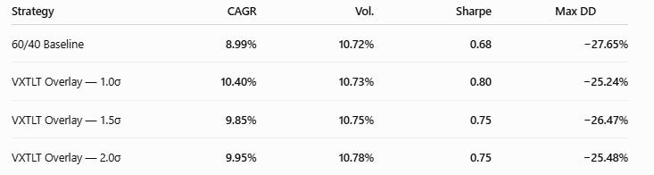
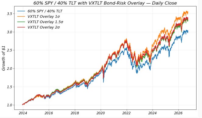
At the 1-standard-deviation threshold, CAGR increases from 8.99% to 10.40%, while the Sharpe ratio rises from 0.68 to 0.80. Maximum drawdown also improves somewhat from about−27% to −25%.
Daily Close Signal: Open-to-Close
As mentioned, the previous close-to-close signal is not fully implementable since it relies on information at the close to trade on the close.
As an alternative, I observe the official VXTLT close on day t, wait until the following day’s open, and, when the signal is active, move the TLT allocation to cash for that trading session. TLT is repurchased at the following close.
The portfolio therefore retains its normal TLT exposure overnight but moves its TLT allocation to cash during the next day, should the signal trigger.
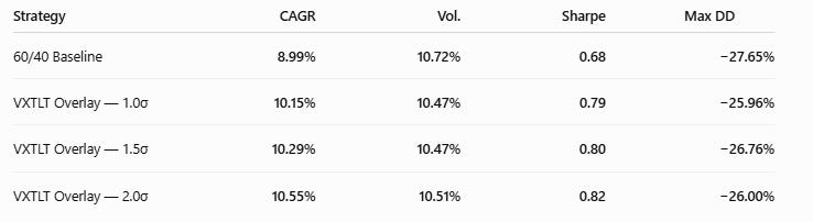
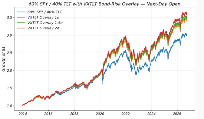
Interestingly, the effect survives this delay. At the 2-standard-deviation threshold, CAGR reaches 10.55%, and the Sharpe ratio rises to 0.82, compared to a Sharpe of 0.68 for the standard 60/40 portfolio.
The year-by-year results are considerably less uniform, however. In particular, much of the improvement in this delayed-execution version is concentrated in 2020.
15:45 Signal: Close-to-Close
Finally, I construct an explicitly pre-close version of the signal using 5-minute VXTLT data.
Instead of waiting for the official close, I observe VXTLT at 15:45 ET and calculate:
The historical mean and standard deviation are still based only on prior daily VXTLT changes.
The signal is therefore known before the market close and can be implemented using market-on-close orders. The resulting position is held from that day’s close until the following close. The sample is shorter because 5-minute VXTLT data are available only from May 2020.
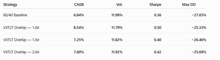
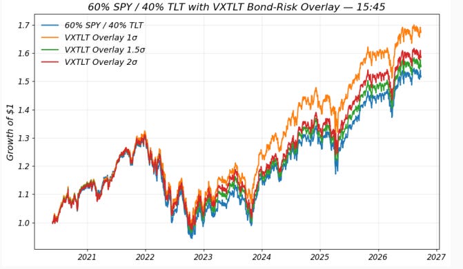
The shorter sample makes this a less powerful test, but the basic result survives in a directly implementable specification. At the 1-standard-deviation threshold, CAGR increases from 6.84% to 8.54%, the Sharpe ratio improves from 0.36 to 0.50, and maximum drawdown again improves somewhat from −27% to −25%.
Interpretation
The results are directionally consistent across the execution assumptions and signal thresholds, although these are variations of the same underlying signal rather than independent tests.
Across the three execution assumptions and three signal thresholds, all nine net-of-cost overlays improve CAGR, Sharpe ratio, and maximum drawdown relative to their corresponding 60/40 baseline.
Large increases in implied Treasury volatility seem to identify periods when Treasury exposure is less attractive over the following trading day.
The result is consistent with the paper’s empirical finding, which is somewhat surprising given the conventional view of Treasuries as a hedge during periods of market stress.
Some of the largest improvements occur during stressed bond-market periods, notably 2020 and 2022, which is consistent with the idea that large volatility shocks can identify periods of unusually poor short-term Treasury returns.
Importantly, the portfolio doesn’t need to forecast the direction of stocks, change its equity allocation, use leverage, or short Treasuries. It simply temporarily removes bond exposure when the implied-volatility signal indicates unusually high short-term Treasury risk.
There are important caveats. The investable VXTLT sample is much shorter than the underlying MOVE evidence in the paper. TLT also represents the long end of the Treasury curve, where the paper’s predictive evidence is weaker than at some shorter maturities. And the signal is explicitly short-term; it should not be interpreted as a long-run Treasury market-timing indicator.
Conclusion
The usual approach to volatility management asks whether investors should hold less of an asset when the level of volatility is high.
For bonds, a potentially more useful question may be:
Is the daily change in bond implied volatility unusually large?
The evidence from VXTLT and TLT suggests that this information can be useful for managing bond exposure over very short horizons.
In my tests, moving from TLT to cash after large increases in Treasury implied volatility improves the performance of a 60/40 portfolio across different thresholds and execution assumptions, even after transaction costs.
The improvement isn’t enormous, and some periods contribute disproportionately.
But for a signal requiring only one volatility index and a simple threshold rule, the consistency across implementations is encouraging.
References
Kodithyala, Siddartha, and Riccardo Rebonato, 2026, Can one volatility-manage fixed-income portfolios?, SSRN Working Paper 7526798.
Disclaimer: This newsletter is for informational and educational purposes only and should not be construed as investment advice. The author does not endorse or recommend any specific securities or investments. While information is gathered from sources believed to be reliable, there is no guarantee of its accuracy, completeness, or correctness.
This content does not constitute personalized financial, legal, or investment advice and may not be suitable for your individual circumstances. Investing carries risks, and past performance does not guarantee future results. The author and affiliates may hold positions in securities discussed, and these holdings may change at any time without prior notification.
The author is not affiliated with, sponsored by, or endorsed by any of the companies, organizations, or entities mentioned in this newsletter. Any references to specific companies or entities are for informational purposes only.
The brief summaries and descriptions of research papers and articles provided in this newsletter should not be considered definitive or comprehensive representations of the original works. Readers are encouraged to refer to the original sources for complete and authoritative information.
This newsletter may contain links to external websites and resources. The inclusion of these links does not imply endorsement of the content, products, services, or views expressed on these third-party sites. The author is not responsible for the accuracy, legality, or content of external sites or for that of any subsequent links. Users access these links at their own risk.
The author assumes no liability for losses or damages arising from the use of this content. By accessing, reading, or using this newsletter, you acknowledge and agree to the terms outlined in this disclaimer.
Paid subscriptions may not be available in all jurisdictions and may change without notice.