Turn-of-the-Month Strategies: Do They Still Work?

Examining the Evidence, Recent Trends, and Practical Implications of a Fading Market Anomaly

Introduction

Decades of research have uncovered numerous market anomalies, persistent patterns in asset returns that cannot be fully explained by traditional risk-based models. Among the most enduring and well-documented of these is the turn-of-the-month (TOM) effect, characterized by abnormally high stock returns during the days surrounding the turn of the calendar month. Unlike other seasonality effects that might be dismissed as mere statistical artifacts, the TOM effect has been consistently observed across various time periods, regions, and even asset classes, sparking interest in its underlying causes and implications for investors.

In this blog post, I explore the key findings on the TOM effect, discuss the potential explanations driving it, and test whether this phenomenon remains relevant in today’s markets.

Contents

• Background

• Testing the TOM effect

  • Data

  • Results for the first TOM Window

  • Results for the second TOM Window

  • TOM Strategies

    • Results for U.S. ETFs

    • Results for International ETFs

• Conclusions

Background

The turn-of-the-month (TOM) effect refers to the tendency for stock market returns to be abnormally strong around the end of the month compared to the rest of the month. The seminal paper by Ariel (1987) was the first to document this phenomenon in U.S. equity markets, showing that nearly all of the monthly excess returns were concentrated in a 9-day window, spanning from the last trading day of the month to eight days later. In contrast, returns during the second half of the month were found to be close to zero.

Building on Ariel’s findings, Lakonishok and Smidt (1988) studied U.S. equity markets over a 90-year period, from 1897 to 1986. They confirmed that end-of-month returns were statistically different from those on other days. Moreover, they identified a narrower 4-day TOM window, starting with the last trading day of the month and extending three days forward, where most of the TOM effect occurred. During this period, average daily returns were estimated at approximately 12 basis points, while returns on all other days were close to zero.

Subsequent studies have largely adopted this 4-day TOM window as the standard definition. For example, Kunkel, Compton, and Beyer (2003) documented a global 4-day TOM effect across 19 countries, while McConnell and Xu (2008) demonstrated that the effect persisted between 1987 and 2005 in both U.S. and international stock markets. Importantly, they found that the TOM effect could not be explained by other seasonal anomalies.

Chen et al. (2015) extended this analysis to international iShares ETFs, finding a pronounced TOM effect between 1996 and 2012. During the TOM window, daily returns averaged 15–20 basis points, while returns on all other days were close to zero. McGroarty et al. (2019) further studied the TOM effect over the period 1961 to 2015, showing that a strategy of being long during the TOM window provided diversification benefits when added to traditional equity and bond portfolios, owing to its low correlation with standard asset classes.

More recently, Etula et al. (2020) broadened the traditional TOM window to 7-days, spanning 3 days before the last trading day to 3 days after ([-3:3]). Their study, covering the period 1995 to 2013, argues that this expanded window better captures the liquidity-driven price impacts of institutional trading. They show that institutions are net sellers during days 0-8 to 0-4, raising cash to meet predictable month-end obligations such as redemptions. This selling pressure peaks on day 0-4 due to the T+3 U.S. settlement convention, resulting in negative returns during the pre-TOM period.

During days 0-3 to 0+3, prices are shown to revert due to the cessation of selling pressure and the onset of buying pressure as new cash inflows are reinvested, driving positive TOM returns. The paper provides causal evidence linking the TOM effect to institutional liquidity needs and settlement conventions, reinforcing the long-held view that the anomaly is driven by predictable investor flows rather than pure randomness.

Below, I plot the average daily return around the end of the month for SPY since its inception, using data from EODHD. The dynamics described by Etula et al. (2020) are evident, with selling pressure during days 0-8 to 0-4 leading to negative returns, followed by a subsequent positive reversal and buying pressure starting on day 0-3. Interestingly, while the broader pattern holds, the day 0 return is negative on average in this sample.

Testing the TOM effect

Let’s test the TOM effect using the most recent data. To maintain consistency with previous studies, I consider two different TOM windows. The first window is the 4 days covering day 0 to day 0+3 ([0:3]), which is the most commonly used definition in the literature. The second window follows the broader definition proposed by Etula et al. (2020), spanning 7 days from day 0-3 to 0+3 ([-3:3]). While the primary focus is on equities, I also include results for other asset classes.

Data

I use daily price data from EODHD, selecting the longest possible time series available for each ETF. For excess return and Sharpe ratio calculations, I use the 3-month T-bill rate (DTB3) sourced from FRED, the Federal Reserve Bank of St. Louis. The analysis covers the following ETFs:

• Equity indices:

SPY - S&P 500

QQQ - Nasdaq 100

IWM - Russell 2000

• Equity sectors:

XLC - Communication Services

XLY - Consumer Discretionary

XLP - Consumer Staples

XLE - Energy

XLF - Financials

XLV - Health Care

XLI - Industrials

XLB - Materials

XLRE - Real Estate

XLK - Technology

XLU - Utilities

• International ETFs (following Chen et al., 2015):

EWA - Australia

EWZ - Brazil

EWC - Canada

EWQ - France

EWG - Germany

EWH - Hong Kong

EWJ - Japan

EWD - Sweden

EWU - U.K.

• Other asset classes:

TLT - iShares 20+ Treasury Bond

HYG - iShares iBoxx High Yield Corporate Bond

UUP - Invesco DB US Dollar Index Bullish Fund

DBA - Invesco DB Agriculture

DBB - Invesco DB Base Metals

DBE - Invesco DB Energy

DBP - Invesco DB Precious Metals

BTC - Bitcoin

I compute the average daily returns for each TOM window and all other days and then calculate the difference between these two. Statistically significant differences are highlighted in bold. The key columns for assessing the TOM anomaly are the last two columns, “Difference %” and “T-stat Difference.”

Results for the First TOM window, [0:3]

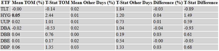
The tables suggest that, while returns during the TOM window are typically a few basis points higher than on other days for equities, none of these differences are statistically significant. The only exceptions are a few international ETFs, specifically those representing Brazil, Canada, and Hong Kong. Assets outside of equities show no evidence of a TOM effect. This lack of a statistically significant TOM effect stands in sharp contrast to findings from earlier studies, which analyzed data up to 2015. Since then, the effect appears to have disappeared, likely arbitraged away by market participants. This decline over the past decade becomes evident when examining a rolling average of the differences in returns.

QQQ exhibited a very strong TOM effect in the early 2000s, but this effect has gradually diminished to zero over time. In contrast, IWM has displayed an opposite TOM effect for many years, with returns during the TOM window underperforming those on other days. A similar downward trend is observed among sector ETFs, where many sectors in recent years also show a negative difference, an inverse TOM effect.

Thus, the classical definition of the TOM effect, measured during the [0:3] window as established by Lakonishok and Smidt (1988), has largely disappeared over the past decade, with TOM returns now indistinguishable from returns on other days. Next, let’s test the broader 7-day window, suggested by Etula et al. (2020).

Results for the Second TOM window, [-3:3]

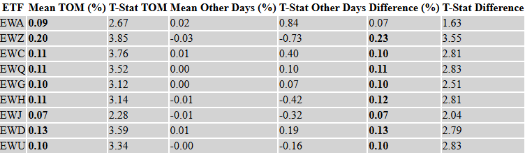
When testing the broader TOM window, most equity ETFs show evidence of a statistically significant TOM effect. Daily average returns tend to be approximately 5–12 basis points higher than on other days, representing an economically meaningful impact. International ETFs exhibit the strongest effects overall, with Brazil showing a particularly notable 23-basis-point difference in returns. Consistent with many other anomalies, the TOM effect appears to be more pronounced in emerging markets. Assets outside of equities show no evidence of the TOM effect, except for high-yield bonds (HYG) and possibly Bitcoin.

Plotting the TOM effect over time reveals that, while it has fluctuated, there has been a consistent downtrend over the last decade, mirroring the decline observed in the classical TOM effect discussed earlier.

Overall, the broader TOM window of [-3:3] produces a statistically significant TOM effect in most equity markets. However, this effect has declined substantially over the past decade.

TOM Strategies

To evaluate the broader TOM effect, let’s examine the performance of long-only strategies that enter at the close on day 0-4 and exit at the close on day 0+3, to capture returns during the [-3:3] window. For simplicity, I assume the strategy earns zero returns when in cash, which understates its performance. Additionally, a one-way transaction cost of 5 basis points is factored into the analysis.

Results for US ETFs

For these three highly liquid markets, going long around the end of the month results in a noticeable drop in CAGR and generally lower or comparable Sharpe ratios. However, the TOM strategy significantly reduces drawdowns, and the drawdown-to-volatility ratio is typically better, except for QQQ. Additionally, TOM strategies exhibit better skewness, measured here on monthly returns. As such, a TOM investor would experience meaningful reductions in CAGR and Sharpe ratios compared to a buy-and-hold approach, while benefiting from improved skewness and lower drawdowns relative to volatility.

Results for International ETFs

As noted earlier, the TOM effect is more pronounced in international markets than in the U.S., though it has also declined over time. For brevity, I report results for the three markets with the most significant TOM effects: Brazil (EWZ), Sweden (EWD), and Hong Kong (EWH).

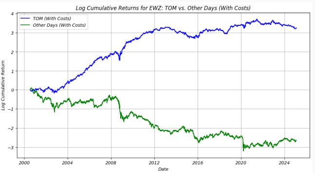
As shown above, some international markets exhibit economically significant TOM effects. Both the CAGR and Sharpe ratios during the TOM window are notably higher than those achieved through a buy-and-hold strategy or on other days.

Conclusions

As with many published anomalies, the classical Turn-of-the-Month (TOM) effect, originally defined as the period from the last trading day of the month to three days after, appears to have largely disappeared in the past decade. This decline suggests that the effect has likely been arbitraged away, consistent with the lifecycle of many anomalies once they are widely publicized and exploited by investors. In particular, U.S. equity markets have shown little evidence of a statistically significant TOM effect in recent years, with returns during the TOM window becoming indistinguishable from those on other days. Notably, some sectors and smaller-cap indices even exhibit a reversal of the effect, with lower returns during the TOM window compared to the rest of the month.

However, expanding the TOM window to include a broader seven-day period, spanning three days before to three days after the last trading day, reveals that the effect persists in a more nuanced form. This broader window, as argued by recent research, better captures the institutional liquidity-driven price impact that contributes to the TOM effect, including pre-month-end selling pressure and subsequent reversal and buying pressure. The effect remains particularly pronounced in international and emerging markets, which are typically less efficient and more susceptible to institutional flows.

These findings highlight both opportunities and challenges for investors. While the TOM effect in U.S. markets may be less appealing as a viable strategy, the broader [-3:3] window suggests there are still pockets of opportunity in less efficient international and emerging markets. However, these strategies must account for transaction costs, which can significantly erode returns, particularly in smaller or less liquid markets. Moreover, the lower drawdowns and improved skewness associated with TOM strategies could offer diversification benefits when incorporated into broader portfolios.

Ultimately, the weakening of the TOM effect underscores the nature of market efficiency and investor behavior, emphasizing that anomalies are rarely permanent and often fade as markets adapt.

---

---

References

Ariel, Robert A., 1987, A monthly effect in stock returns, Journal of Financial Economics 18, 161-174.

Chen, Haiwei, Sang Heon Shin, and Xu Sun, 2015, Return-enhancing strategies with international ETFs: Exploiting the turn-of-the-month effect, Financial Services Review 24, 271-288.

Etula, Erkko, Kalle Rinne, Matti Suominen, and Lauri Vaittinen, 2020, Dash for cash: Monthly market impact of institutional liquidity needs, Review of Financial Studies 33, 75-111.

Kunkel, Robert A., William S. Compton, and Scott Beyer, 2003, The turn-of-the-month effect still lives: the international evidence, International Review of Financial Analysis 12, 207-221.

Lakonishok, Josef, and Seymour Smidt, 1988, Are seasonal anomalies real? A ninety-year perspective, Review of Financial Studies 1, 403-425.

McConnell, John J., and Wei Xu, 2008, Equity returns at the turn of the month, Financial Analyst Journal 64, 49-64.

McGroarty, Frank, Emmanouil Platanakis, Athanasios Sakkas, and Andrew Urquhart, 2019, A seasonality factor in asset allocation, SSRN Working Paper 3266285.

---

Disclaimer: This article is for informational and educational purposes only and should not be construed as investment advice. The author does not endorse any specific securities or investments mentioned. While information is gathered from sources believed to be reliable, there is no guarantee of its accuracy, completeness, or correctness.

This content does not offer personalized financial, legal, or investment advice and may not be suitable for your individual circumstances. Investing carries risks, and past performance does not guarantee future results. The author and affiliates may hold positions in securities discussed without prior notification.

The author is not affiliated with, sponsored by, or endorsed by any of the companies, organizations, or entities mentioned in this newsletter. Any references to specific companies or entities are for informational purposes only.

The brief summaries and descriptions of research papers and articles provided in this article are the author's own interpretations of the findings and content. These summaries should not be considered as definitive or comprehensive representations of the original works. Readers are encouraged to refer to the original sources for complete and authoritative information.